Transient Two-Node Model

A diffusive node with internal dissipation heats up against a cold boundary, exchanging heat through conductive and radiative couplings.

The example also demonstrates a simple manual sensitivity comparison by re-running with a doubled conductive coupling.

Build the baseline model

import matplotlib.pyplot as plt

from pycanha.solvers import TSCNRLDS
from pycanha.tmm import Node, NodeType, ThermalMathematicalModel

tmm = ThermalMathematicalModel("TwoNodeTransient")

node1 = Node(1)
node1.T = 273.0
node1.C = 1.0e4
node1.qi = 500.0

node2 = Node(2)
node2.T = 3.0
node2.type = NodeType.BOUNDARY

tmm.add_node(node1)
tmm.add_node(node2)
tmm.conductive_couplings.add_coupling(1, 2, 0.5)
tmm.radiative_couplings.add_coupling(1, 2, 1.0e-7)

Solve the transient

start, end, dt, out_dt = 0.0, 200_000.0, 1_000.0, 5_000.0

solver = TSCNRLDS(tmm)
solver.set_simulation_time(start, end, dt, out_dt)
solver.initialize()
solver.solve()

output_model = tmm.thermal_data.models.get_model(solver.output_model_name)
times = output_model.T.times
idx1 = tmm.nodes.get_idx_from_node_num(1)
T1 = output_model.T.values[:, idx1]

Sensitivity run — doubled conductance

tmm2 = ThermalMathematicalModel("HighGL")
n1b = Node(1)
n1b.T = 273.0
n1b.C = 1.0e4
n1b.qi = 500.0
n2b = Node(2)
n2b.T = 3.0
n2b.type = NodeType.BOUNDARY
tmm2.add_node(n1b)
tmm2.add_node(n2b)
tmm2.conductive_couplings.add_coupling(1, 2, 1.0)
tmm2.radiative_couplings.add_coupling(1, 2, 1.0e-7)

solver2 = TSCNRLDS(tmm2)
solver2.set_simulation_time(start, end, dt, out_dt)
solver2.initialize()
solver2.solve()

output_model2 = tmm2.thermal_data.models.get_model(solver2.output_model_name)
T1b = output_model2.T.values[:, tmm2.nodes.get_idx_from_node_num(1)]

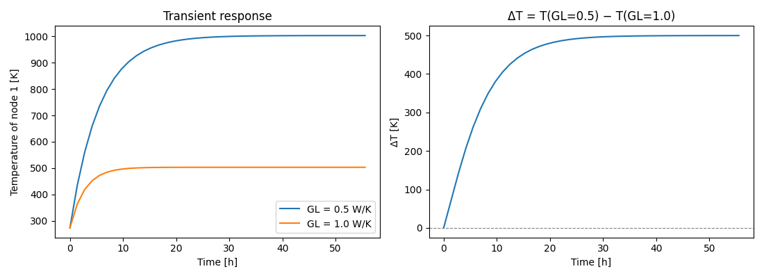
Plot

fig, axes = plt.subplots(1, 2, figsize=(11, 4))

axes[0].plot(times / 3600, T1, label="GL = 0.5 W/K")
axes[0].plot(times / 3600, T1b, label="GL = 1.0 W/K")
axes[0].set_xlabel("Time [h]")
axes[0].set_ylabel("Temperature of node 1 [K]")
axes[0].set_title("Transient response")
axes[0].legend()

axes[1].plot(times / 3600, T1 - T1b)
axes[1].axhline(0, color="gray", linewidth=0.8, linestyle="--")
axes[1].set_xlabel("Time [h]")
axes[1].set_ylabel("ΔT [K]")
axes[1].set_title("ΔT = T(GL=0.5) − T(GL=1.0)")

plt.tight_layout()
plt.show()