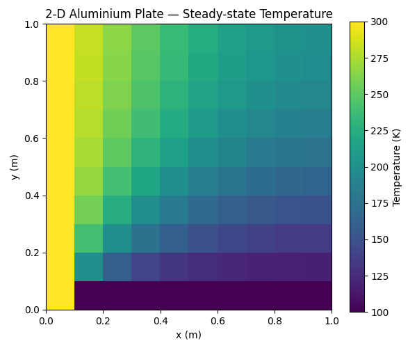
Steady-State 2D Plate

Solve the temperature distribution of a 2D aluminium plate with fixed boundary conditions on two edges.

• Left edge (i = 1): T = 300 K (hot)

• Bottom edge (j = 1): T = 100 K (cold)

• Right and top edges: adiabatic (no heat flow)

• Interior and remaining edges: diffusive

Model setup

We use a 10 × 10 grid of thermal nodes connected by conductive couplings derived from the aluminium thermal conductivity.

import matplotlib.pyplot as plt
import numpy as np

from pycanha.solvers import SSLU
from pycanha.tmm import Node, NodeType, ThermalMathematicalModel

# Physical data
Lx, Ly = 1.0, 1.0  # plate dimensions [m]
t_plate = 1e-2  # thickness [m]
k_Al = 180.0  # thermal conductivity [W/(m·K)]

# Mesh
Nx, Ny = 10, 10

tmm = ThermalMathematicalModel(name="AluPlate")

for j in range(1, Ny + 1):
    for i in range(1, Nx + 1):
        node_num = i + (j - 1) * Nx
        node = Node(node_num)
        if i == 1 or j == 1:
            node.type = NodeType.BOUNDARY
        tmm.add_node(node)

Conductive couplings

coupling_value = k_Al * t_plate / (Lx / (Nx - 1))

# Horizontal
for j in range(1, Ny + 1):
    for i in range(1, Nx):
        tmm.conductive_couplings.add_coupling(
            i + (j - 1) * Nx, (i + 1) + (j - 1) * Nx, coupling_value
        )

# Vertical
for j in range(1, Ny):
    for i in range(1, Nx + 1):
        tmm.conductive_couplings.add_coupling(i + (j - 1) * Nx, i + j * Nx, coupling_value)

Boundary temperatures

for j in range(1, Ny + 1):
    for i in range(1, Nx + 1):
        node_num = i + (j - 1) * Nx
        if i == 1:
            tmm.nodes.set_T(node_num, 300.0)
        elif j == 1:
            tmm.nodes.set_T(node_num, 100.0)

Solve and plot

solver = SSLU(tmm)
solver.initialize()
solver.solve()

temp_matrix = np.zeros((Ny, Nx))
for j in range(1, Ny + 1):
    for i in range(1, Nx + 1):
        temp_matrix[j - 1, i - 1] = tmm.nodes.get_T(i + (j - 1) * Nx)

plt.figure(figsize=(6, 5))
plt.imshow(
    temp_matrix,
    cmap="viridis",
    origin="lower",
    extent=[0, Lx, 0, Ly],
    aspect="equal",
)
plt.colorbar(label="Temperature (K)")
plt.xlabel("x (m)")
plt.ylabel("y (m)")
plt.title("2-D Aluminium Plate — Steady-state Temperature")
plt.tight_layout()
plt.show()