Build a thermal model from an ESATAN TMD file

There are two different TMD readers in pycanha:

1. from_esatan_tmd() (this example) builds a full thermal model from the file: it creates the nodes and loads, and both the conductive (GL) and radiative (GR) couplings. The result is a solvable model.

2. read_tmd_transient (next example) only reads time-dependent result data into a data container; it does not build a model.

Here we build the disc in a spherical enclosure model from its steady-state .TMD results file, retrieve some couplings, solve the steady state, and run a transient analysis. The disc is a 100 nodes Delrin disc (nodes 1000-1099). 10 W is dissipated in a middle ring and radiated to a boundary at -10 degC.

Locate the model file and build the model

from_esatan_tmd returns a ThermalModel object.

from pathlib import Path

import matplotlib.pyplot as plt
import numpy as np
import pycanha_core as pcc

import pycanha as pc

# The C++ core logs solver progress at INFO, quiet it for cleaner output.
pcc.set_logger_level(pcc.LogLevel.WARN)

# Resolve the test data path.
_cwd = Path.cwd()
_DATA = next(
    p / "tests" / "data" / "esatan" / "DISC"
    for p in (_cwd, *_cwd.parents)
    if (p / "tests" / "data" / "esatan" / "DISC").is_dir()
)
STEADY = _DATA / "DISCTR_STEADY.TMD"

model = pc.ThermalModel.from_esatan_tmd(str(STEADY), name="disc")
nodes = model.tmm.nodes
node_numbers = [nodes.get_node_num_from_idx(i) for i in range(nodes.num_nodes)]
print(f"{nodes.num_nodes} nodes built (disc 1000-1099 + boundary 2000, 99999)")

102 nodes built (disc 1000-1099 + boundary 2000, 99999)

Retrieve the couplings (GL / GR)

Conductive (GL) and radiative (GR) couplings are queried by node number pair with get_coupling_value. We also enumerate them all.

cc = model.tmm.conductive_couplings
rc = model.tmm.radiative_couplings

print("GL(1000, 1001) =", cc.get_coupling_value(1000, 1001), "W/K")
print("GR(1000, 1002) =", rc.get_coupling_value(1000, 1002))

gl_couplings, gr_couplings = [], []
for a, i in enumerate(node_numbers):
    for j in node_numbers[a + 1 :]:
        g = cc.get_coupling_value(i, j)
        if g:
            gl_couplings.append((i, j, g))
        r = rc.get_coupling_value(i, j)
        if r:
            gr_couplings.append((i, j, r))

print(
    f"{len(gl_couplings)} conductive (GL) couplings, {len(gr_couplings)} radiative (GR) couplings"
)

GL(1000, 1001) = 0.0029000000000000002 W/K
GR(1000, 1002) = 6.25351e-09
190 conductive (GL) couplings, 5050 radiative (GR) couplings

Solve the steady-state and recover the temperatures

The file already stores ESATAN’s converged temperatures. We overwrite every non boundary node with a wrong value, solve the steady state ourselves, and check the original temperatures come back.

def disc_temperatures_celsius():
    return {
        nodes.get_node_num_from_idx(i): nodes.get_node_from_idx(i).T - 273.15
        for i in range(nodes.num_nodes)
    }


reference = disc_temperatures_celsius()  # ESATAN's stored solution

# Perturb: force every non-boundary node to 0 degC.
for i in range(nodes.num_nodes):
    if nodes.get_node_num_from_idx(i) not in (2000, 99999):
        nodes.get_node_from_idx(i).T = 273.15

solver = model.solvers.sslu
solver.max_iters = 100
solver.abstol_temp = 1e-4
solver.initialize()
solver.solve()

recovered = disc_temperatures_celsius()
max_diff = max(abs(recovered[n] - reference[n]) for n in reference)
print(f"max |recovered - reference| = {max_diff:.2e} degC")
print(f"peak disc temperature = {max(reference.values()):.2f} degC")

max |recovered - reference| = 2.97e-07 degC
peak disc temperature = 120.07 degC

Run a transient analysis

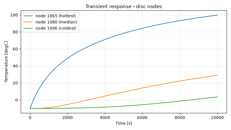
Start everything at -10 degC and integrate for 10 000 s with the Crank-Nicolson solver. We then plot three disc nodes (no environment nodes).

for i in range(nodes.num_nodes):
    if nodes.get_node_num_from_idx(i) != 99999:
        nodes.get_node_from_idx(i).T = 273.15 - 10.0

solver = model.solvers.tscnrlds
solver.max_iters = 100
solver.abstol_temp = 1e-7
solver.set_simulation_time(0.0, 10000.0, 1.0, 100.0)
solver.initialize()
solver.solve()

output = solver.output_model
times = np.asarray(output.T.times)
temperatures = np.asarray(output.T.values)
column_of = {node: i for i, node in enumerate(output.node_numbers)}

Plot the transient response

disc_nodes = [n for n in output.node_numbers if 1000 <= n <= 1099]
final = {n: temperatures[-1, column_of[n]] for n in disc_nodes}
picks = [
    (max(final, key=final.get), "hottest"),
    (sorted(disc_nodes, key=lambda n: final[n])[len(disc_nodes) // 2], "median"),
    (min(final, key=final.get), "coldest"),
]

plt.figure(figsize=(8, 4.5))
for node, label in picks:
    plt.plot(times, temperatures[:, column_of[node]] - 273.15, label=f"node {node} ({label})")
plt.xlabel("Time [s]")
plt.ylabel("Temperature [degC]")
plt.title("Transient response - disc nodes")
plt.legend()
plt.grid(alpha=0.3)
plt.tight_layout()
plt.show()