Parametric analysis

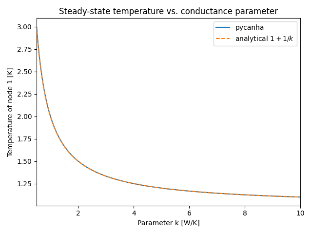
Sweep the conductive coupling parameter k and compare the computed steady-state temperature against the analytical solution \(T_1 = T_2 + q_i / k\).

This example demonstrates the Parameters and ParameterFormula API.

Build model with a parametric coupling

import matplotlib.pyplot as plt
import numpy as np

import pycanha as pc
import pycanha.tmm as pm

tm = pc.ThermalModel("Parametric")
tmm = tm.tmm

node1 = pm.Node(1)
node1.C = 1.0
node1.qi = 1.0

node2 = pm.Node(2)
node2.T = 1.0
node2.type = pm.NodeType.BOUNDARY

tmm.add_node(node1)
tmm.add_node(node2)
tmm.conductive_couplings.add_coupling(1, 2, 1.0)

# Link GL(1,2) to parameter "k"
tmm.parameters.add_parameter("k", 1.0)
tmm.formulas.add_formula("GL(1,2)", "k")

<pycanha_core.pycanha_core.parameters.ParameterFormula object at 0x75d7f62b1450>

Sweep the coupling parameter

solver = tm.solvers.sslu
solver.initialize()

k_values = np.linspace(0.5, 10.0, 200)
T_results = np.empty_like(k_values)

for i, k in enumerate(k_values):
    tmm.parameters.set_parameter("k", k)
    tmm.formulas.apply_formulas()
    solver.solve()
    T_results[i] = tmm.nodes.get_T(1)

solver.deinitialize()

Compare with analytical solution

T_analytical = 1.0 + 1.0 / k_values

plt.figure()
plt.plot(k_values, T_results, label="pycanha")
plt.plot(k_values, T_analytical, "--", label=r"analytical $1 + 1/k$")
plt.xlabel("Parameter k [W/K]")
plt.ylabel("Temperature of node 1 [K]")
plt.title("Steady-state temperature vs. conductance parameter")
plt.xlim(k_values[0], k_values[-1])
plt.legend()
plt.tight_layout()
plt.show()