Transient correlation of the simple 4-node model

This example reproduces the Simple 4-nodes model from

J. Piqueras, et al., “Efficient transient correlation of thermal lumped network models to reference data”, Acta Astronautica 210 (2023).

The model (Fig. 3) has three diffusive nodes (1, 2, 3) and one boundary node (4) held at 20 °C. A 100 W load is applied to node 1. Nodes are linked by conductive couplings GL(1,2), GL(1,3), GL(1,4) and radiative couplings GR(2,3), GR(2,4), GR(3,4).

The goal is to recover a set of reference parameter values starting from a perturbed base set, by correlating the transient response. The correlation is a non-linear least-squares problem whose Jacobian dT/dp is provided by the Jacobian Propagation method described in the paper and implemented in the TSCNRLDS_JACOBIAN solver, so no finite differences are needed.

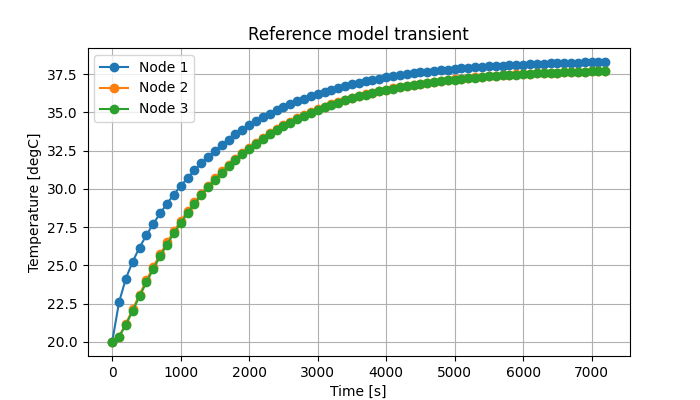
Build the model and generate the reference data

We build the 4-node model, drive every free parameter with a formula, set the parameters to their reference values, run the (non-Jacobian) TSCNRLDS transient solver, store the reference temperatures, and plot them.

import contextlib
import os

import matplotlib.pyplot as plt
import numpy as np
import pycanha_core as pcc
from scipy.optimize import least_squares

import pycanha as pc
import pycanha.tmm as pm

# Silence the C++ info logger.
pcc.set_logger_level(pcc.OFF)


# The solver's separate "profiling" logger writes straight to the OS stdout,
# so it is not affected by set_logger_level. This small context manager
# redirects the stdout file descriptor to null while a solver runs, keeping
# the example output clean. (Simple, repetitive-use helper.)
@contextlib.contextmanager
def silence():
    devnull = os.open(os.devnull, os.O_WRONLY)
    saved_stdout = os.dup(1)
    os.dup2(devnull, 1)
    try:
        yield
    finally:
        os.dup2(saved_stdout, 1)
        os.close(devnull)
        os.close(saved_stdout)


# --- Problem constants ---
KELVIN = 273.15
T0 = 20.0 + KELVIN  # initial temperature of every node and boundary value [K]
Q1 = 100.0  # heat load applied to node 1 [W]
DT = 100.0  # time step [s]
T_END = 7200.0  # end time [s]
ABSTOL = 1e-5  # temperature convergence tolerance [K]

# Free parameters (Table 1). Names must NOT look like entities (e.g. "C1"),
# hence the "par_" prefix. REFERENCE = true values, BASE = perturbed start.
PARAM_NAMES = [
    "par_c1",
    "par_c2",
    "par_c3",
    "par_gl12",
    "par_gl13",
    "par_gl14",
    "par_gr24",
    "par_gr23",
    "par_gr34",
]
LABELS = ["C1", "C2", "C3", "GL12", "GL13", "GL14", "GR24", "GR23", "GR34"]
REFERENCE = np.array([3000.0, 2500.0, 2000.0, 8.0, 6.0, 5.0, 0.04, 0.08, 0.03])
BASE = np.array([3570.0, 850.0, 1600.0, 2.0, 1.0, 4.0, 0.03, 0.05, 0.08])

# --- Build the 4-node model ---
model = pc.ThermalModel("simple_4node")
tmm = model.tmm

# Three diffusive nodes, all starting at 20 degC.
for node_num in (1, 2, 3):
    node = pm.Node(node_num)
    node.type = pm.NodeType.DIFFUSIVE
    node.T = T0
    node.capacity = 1.0  # placeholder; overwritten by the capacity formula
    tmm.add_node(node)

# 100 W applied to node 1 as internal dissipation.
tmm.nodes.get_node_from_node_num(1).qi = Q1

# Node 4 is the boundary heat sink held at 20 degC.
boundary = pm.Node(4)
boundary.type = pm.NodeType.BOUNDARY
boundary.T = T0
tmm.add_node(boundary)

# Couplings must exist before a formula can target them; the placeholder value
# 1.0 is immediately overwritten by apply_formulas().
tmm.add_conductive_coupling(1, 2, 1.0)
tmm.add_conductive_coupling(1, 3, 1.0)
tmm.add_conductive_coupling(1, 4, 1.0)
tmm.add_radiative_coupling(2, 4, 1.0)
tmm.add_radiative_coupling(2, 3, 1.0)
tmm.add_radiative_coupling(3, 4, 1.0)

# Link each parameter to its entity and flag it for derivative computation.
ent = tmm.entities
entities = [
    ent.capacity(1),
    ent.capacity(2),
    ent.capacity(3),
    ent.conductive_coupling(1, 2),
    ent.conductive_coupling(1, 3),
    ent.conductive_coupling(1, 4),
    ent.radiative_coupling(2, 4),
    ent.radiative_coupling(2, 3),
    ent.radiative_coupling(3, 4),
]
for name, entity, value in zip(PARAM_NAMES, entities, REFERENCE):
    model.parameters.add_parameter(name, float(value))
    tmm.formulas.add_parameter_formula(entity, name)
    tmm.formulas.parameters_with_derivatives.add_parameter(name)

# Push the reference parameter values into the network.
tmm.formulas.apply_formulas()

# --- Simulate the reference model (non-Jacobian transient solver) ---
ref_solver = model.solvers.tscnrlds
ref_solver.abstol_temp = ABSTOL
ref_solver.set_simulation_time(0.0, T_END, DT, DT)
with silence():
    ref_solver.initialize()
    ref_solver.solve()

# Store the reference results: time grid and the 3 diffusive-node temperatures
# (column 4 is the constant boundary node, so we drop it).
times = np.asarray(ref_solver.output_model.T.times).copy()
T_reference = np.asarray(ref_solver.output_model.T.values)[:, :3].copy()

# --- Plot reference temperatures vs time ---
fig, ax = plt.subplots(figsize=(7, 4))
for i in range(3):
    ax.plot(times, T_reference[:, i] - KELVIN, "-o", label=f"Node {i + 1}")
ax.set_xlabel("Time [s]")
ax.set_ylabel("Temperature [degC]")
ax.set_title("Reference model transient")
ax.legend()
ax.grid(True)
plt.show()

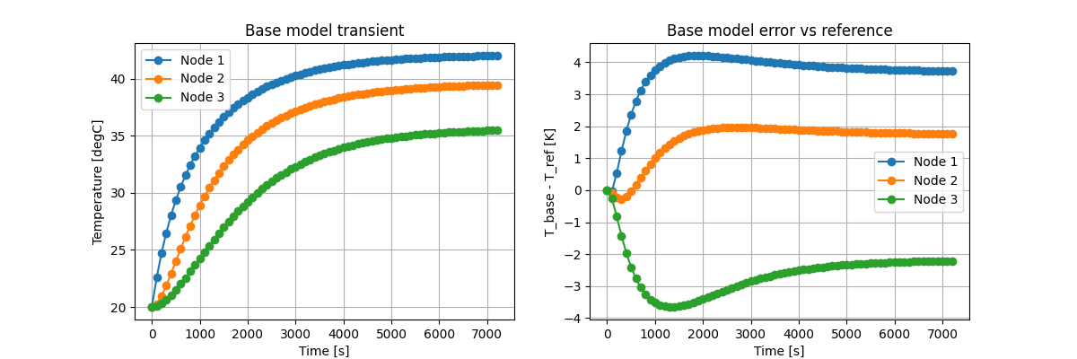
Base model: simulate and compare with the reference

Reusing the same model, we switch the parameters to the perturbed base values, run the transient again, and plot both the base temperatures and the error (base − reference) of the three nodes versus time.

# Set the parameters to the perturbed BASE values and propagate to the network.
for name, value in zip(PARAM_NAMES, BASE):
    model.parameters.set_parameter(name, float(value))
tmm.formulas.apply_formulas()

# The solver writes the final temperatures back into the nodes (Td is an
# Eigen::Map view over the node temperatures), so reset every node to the
# initial condition before solving again.
for node_num in (1, 2, 3, 4):
    tmm.nodes.set_T(node_num, T0)

# Re-run the same (non-Jacobian) solver with the base parameters.
with silence():
    ref_solver.solve()
T_base = np.asarray(ref_solver.output_model.T.values)[:, :3].copy()

# Error of the base model w.r.t. the reference, per node and time.
error_base = T_base - T_reference

# --- Plot base temperatures and the error vs time ---
fig, (ax1, ax2) = plt.subplots(1, 2, figsize=(12, 4))
for i in range(3):
    ax1.plot(times, T_base[:, i] - KELVIN, "-o", label=f"Node {i + 1}")
ax1.set_xlabel("Time [s]")
ax1.set_ylabel("Temperature [degC]")
ax1.set_title("Base model transient")
ax1.legend()
ax1.grid(True)
for i in range(3):
    ax2.plot(times, error_base[:, i], "-o", label=f"Node {i + 1}")
ax2.set_xlabel("Time [s]")
ax2.set_ylabel("T_base - T_ref [K]")
ax2.set_title("Base model error vs reference")
ax2.legend()
ax2.grid(True)
plt.show()

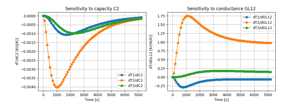
Transient sensitivities (Jacobian solver)

The TSCNRLDS_JACOBIAN solver integrates the model and, at the same time, propagates the derivatives dT/dp of every flagged parameter (Jacobian Propagation). Here we initialize it (the model is still at the base values) and plot the time evolution of the sensitivities of the three node temperatures to one capacity (C2) and one conductance (GL12).

As noted in the paper, all derivatives start at zero (the initial temperatures do not depend on the parameters) and the sensitivity to a thermal capacity tends back to zero at steady state.

# Build and initialize the Jacobian solver (model currently at the base values).
jac_solver = model.solvers.tscnrlds_jacobian
jac_solver.abstol_temp = ABSTOL
jac_solver.max_iters = 50
jac_solver.set_simulation_time(0.0, T_END, DT, DT)
with silence():
    jac_solver.initialize()

# Reset the initial temperatures and solve.
for node_num in (1, 2, 3, 4):
    tmm.nodes.set_T(node_num, T0)
with silence():
    jac_solver.solve()

# The Jacobian column order matches derivative_parameter_names (== PARAM_NAMES).
# Each stored matrix jac.at(k) has shape (3 diffusive nodes, 9 parameters);
# stack over time into J with shape (n_times, 3 nodes, 9 params).
jac = jac_solver.output_model.jacobian
jac_times = np.asarray(jac.times)
J = np.stack([np.asarray(jac.at(k)) for k in range(jac.num_timesteps)])

# Pick one capacity parameter (C2) and one conductance parameter (GL12).
col_c2 = PARAM_NAMES.index("par_c2")
col_gl12 = PARAM_NAMES.index("par_gl12")

fig, (ax1, ax2) = plt.subplots(1, 2, figsize=(12, 4))
for i in range(3):
    ax1.plot(jac_times, J[:, i, col_c2], "-o", label=f"dT{i + 1}/dC2")
ax1.set_xlabel("Time [s]")
ax1.set_ylabel("dT/dC2 [K/(J/K)]")
ax1.set_title("Sensitivity to capacity C2")
ax1.legend()
ax1.grid(True)
for i in range(3):
    ax2.plot(jac_times, J[:, i, col_gl12], "-o", label=f"dT{i + 1}/dGL12")
ax2.set_xlabel("Time [s]")
ax2.set_ylabel("dT/dGL12 [K/(W/K)]")
ax2.set_title("Sensitivity to conductance GL12")
ax2.legend()
ax2.grid(True)
plt.show()

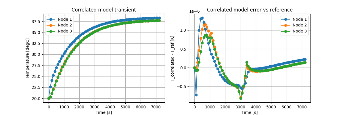
Correlation: recover the reference parameters

We define the least-squares residual and the Jacobian and pass them to scipy.optimize.least_squares (Levenberg–Marquardt). Each residual is the difference between the model and reference temperature of a diffusive node at a time sample. The Jacobian comes directly from the TSCNRLDS_JACOBIAN solver.

Starting from the base values, the optimization process recovers the reference values. Finally we plot the correlated transient and its error versus the reference (now reduced to numerical noise).

# Residual vector: (model - reference) temperatures of the 3 diffusive nodes
# at every time sample, flattened. The Jacobian solver returns both T and
# dT/dp; least_squares calls residuals() and jacobian() at the same x, so we
# (re)solve in each -- the 4-node model is tiny.
def residuals(x):
    for name, value in zip(PARAM_NAMES, x):
        model.parameters.set_parameter(name, float(value))
    tmm.formulas.apply_formulas()
    for node_num in (1, 2, 3, 4):
        tmm.nodes.set_T(node_num, T0)
    with silence():
        jac_solver.solve()
    T_model = np.asarray(jac_solver.output_model.T.values)[:, :3]
    return (T_model - T_reference).reshape(-1)


def jacobian(x):
    for name, value in zip(PARAM_NAMES, x):
        model.parameters.set_parameter(name, float(value))
    tmm.formulas.apply_formulas()
    for node_num in (1, 2, 3, 4):
        tmm.nodes.set_T(node_num, T0)
    with silence():
        jac_solver.solve()
    j = jac_solver.output_model.jacobian
    # Stack the per-time (3 nodes, 9 params) matrices to match the residual
    # ordering (row-major over time then node).
    return np.vstack([np.asarray(j.at(k)) for k in range(j.num_timesteps)])


# Run the non-linear least-squares correlation starting from the base values.
# We use ``trf`` with non-negative bounds because Levenberg-Marquardt can take
# a Newton step into negative parameter territory on the first iteration,
# which makes the radiation matrix indefinite and breaks the linear solve.
result = least_squares(
    residuals,
    BASE.copy(),
    jac=jacobian,
    method="trf",
    bounds=(0.0, np.inf),
    xtol=1e-12,
    ftol=1e-12,
    gtol=1e-12,
)
recovered = result.x

# Evaluate the correlated model.
for name, value in zip(PARAM_NAMES, recovered):
    model.parameters.set_parameter(name, float(value))
tmm.formulas.apply_formulas()
for node_num in (1, 2, 3, 4):
    tmm.nodes.set_T(node_num, T0)
with silence():
    jac_solver.solve()
T_correlated = np.asarray(jac_solver.output_model.T.values)[:, :3].copy()
error_correlated = T_correlated - T_reference

# --- Plot correlated temperatures and the (now tiny) error vs time ---
fig, (ax1, ax2) = plt.subplots(1, 2, figsize=(12, 4))
for i in range(3):
    ax1.plot(times, T_correlated[:, i] - KELVIN, "-o", label=f"Node {i + 1}")
ax1.set_xlabel("Time [s]")
ax1.set_ylabel("Temperature [degC]")
ax1.set_title("Correlated model transient")
ax1.legend()
ax1.grid(True)
for i in range(3):
    ax2.plot(times, error_correlated[:, i], "-o", label=f"Node {i + 1}")
ax2.set_xlabel("Time [s]")
ax2.set_ylabel("T_correlated - T_ref [K]")
ax2.set_title("Correlated model error vs reference")
ax2.legend()
ax2.grid(True)
plt.show()