Steady-state correlation of the PHI-ELE 7-node model

This example reproduces the PHI-ELE example from

I. Torralbo, et al.,
"Correlation of spacecraft thermal mathematical models to reference data",
*Acta Astronautica* **144** (2018).

The PHI-ELE (Polarimetric Helioseismic Imager - Electronics Unit) reduced thermal model has 7 diffusive nodes: four sidewalls (1-4), the top shell (5), the baseplate (6), and the electronics boards (7). Two boundary nodes carry the spacecraft interface: a radiative I/F (90000) and a conductive I/F (90001). Six free conductive parameters x1..x6 group the model’s 17 conductive couplings (Table 6). The five radiative couplings to the spacecraft are fixed and are NOT part of the correlation.

The correlation uses both load cases jointly (C1 hot + C2 cold). The Jacobian is built by forward finite differences around the SSLU steady-state solver.

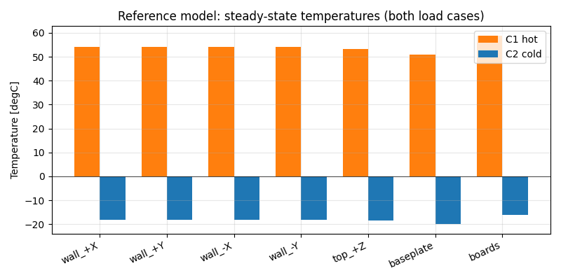
Build the model and generate the reference data

We build the 7-node RTMM, drive every conductance group with a parameter formula, set the parameters to their reference values (Table 7), run the SSLU steady-state solver for both load cases, store the reference temperatures, and plot them.

import contextlib
import os

import matplotlib.pyplot as plt
import numpy as np
import pycanha_core as pcc
from scipy.optimize import least_squares

import pycanha as pc
import pycanha.tmm as pm

# Silence the C++ info logger.
pcc.set_logger_level(pcc.OFF)


# The solver's separate "profiling" logger writes straight to OS stdout, so
# it is not affected by set_logger_level. This small context manager
# redirects the stdout file descriptor to null during a solve, keeping the
# notebook output clean.
@contextlib.contextmanager
def silence():
    devnull = os.open(os.devnull, os.O_WRONLY)
    saved_stdout = os.dup(1)
    os.dup2(devnull, 1)
    try:
        yield
    finally:
        os.dup2(saved_stdout, 1)
        os.close(devnull)
        os.close(saved_stdout)


# --- Problem constants ---
KELVIN = 273.15
ABSTOL = 1e-8  # SSLU Newton iteration tolerance [K]

NODE_NUMS = [1, 2, 3, 4, 5, 6, 7]
NODE_LABELS = ["wall_+X", "wall_+Y", "wall_-X", "wall_-Y", "top_+Z", "baseplate", "boards"]
SC_RAD_NODE = 90000  # boundary: SC radiative I/F
SC_COND_NODE = 90001  # boundary: SC conductive I/F

# Load cases (Table 5). Heat load applied to node 7 (boards) as qi.
CASES = {
    "C1": dict(q7=30.9, T_rad=50.0 + KELVIN, T_cond=48.9 + KELVIN),
    "C2": dict(q7=14.4, T_rad=-20.0 + KELVIN, T_cond=-21.1 + KELVIN),
}

# Free parameters x1..x6 (Table 7 reference values in W/K) and BASE = 0.5 * REF.
PARAM_NAMES = ["par_x1", "par_x2", "par_x3", "par_x4", "par_x5", "par_x6"]
LABELS = ["x1", "x2", "x3", "x4", "x5", "x6"]
REFERENCE = np.array([1.0, 0.225, 1.175, 1.05, 1.4375, 12.2])
BASE = 0.5 * REFERENCE

# Conductive coupling groups (Table 6). Each parameter drives several GLs.
# Sidewall-sidewall is asymmetric in the paper: only k12, k13, k34.
COUPLING_GROUPS = {
    "par_x1": [(1, 2), (1, 3), (3, 4)],  # sidewall - sidewall
    "par_x2": [(1, 5), (2, 5), (3, 5), (4, 5)],  # sidewall - top shell
    "par_x3": [(1, 6), (2, 6), (3, 6), (4, 6)],  # sidewall - baseplate
    "par_x4": [(1, 7), (2, 7), (3, 7), (4, 7)],  # board - sidewall
    "par_x5": [(6, 7)],  # board - baseplate
    "par_x6": [(6, SC_COND_NODE)],  # baseplate - SC cond I/F
}

# Fixed radiative couplings (m^2). NOT correlated.
RAD_COUPLINGS = [
    (1, SC_RAD_NODE, 0.03105),
    (2, SC_RAD_NODE, 0.03105),
    (3, SC_RAD_NODE, 0.03105),
    (4, SC_RAD_NODE, 0.03105),
    (5, SC_RAD_NODE, 0.03060),
]

# --- Build the model ---
model = pc.ThermalModel("phi_ele")
tmm = model.tmm

# Seven diffusive nodes; capacities don't matter for steady state.
for n in NODE_NUMS:
    node = pm.Node(n)
    node.type = pm.NodeType.DIFFUSIVE
    node.T = 293.15  # initial guess; overwritten per load case
    node.capacity = 1.0
    tmm.add_node(node)

# Two boundary nodes (SC interfaces). T is overwritten per load case.
for bn in (SC_RAD_NODE, SC_COND_NODE):
    b = pm.Node(bn)
    b.type = pm.NodeType.BOUNDARY
    b.T = 293.15
    tmm.add_node(b)

# Placeholder conductive couplings (formulas overwrite the value).
for pairs in COUPLING_GROUPS.values():
    for n1, n2 in pairs:
        tmm.add_conductive_coupling(n1, n2, 1.0)

# Fixed radiative couplings.
for n1, n2, gr in RAD_COUPLINGS:
    tmm.add_radiative_coupling(n1, n2, gr)

# Parameters + formulas: each x_i drives every GL in its group.
for name, value in zip(PARAM_NAMES, REFERENCE):
    model.parameters.add_parameter(name, float(value))
    for n1, n2 in COUPLING_GROUPS[name]:
        entity = tmm.entities.conductive_coupling(n1, n2)
        tmm.formulas.add_parameter_formula(entity, name)

tmm.formulas.apply_formulas()


# --- Initialize the SSLU steady-state solver ---
sslu = model.solvers.sslu
sslu.abstol_temp = ABSTOL
with silence():
    sslu.initialize()


# --- Tiny helper to solve one load case (sanctioned repetitive task) ---
def solve_case(case):
    """Configure a load case (boundary temperatures + node-7 heat load),
    reset the diffusive node temperatures to a sensible initial guess, run
    SSLU, and return the 7-node temperature vector [K]."""
    tmm.nodes.set_T(SC_RAD_NODE, case["T_rad"])
    tmm.nodes.set_T(SC_COND_NODE, case["T_cond"])
    tmm.nodes.set_qi(7, case["q7"])
    init_T = 0.5 * (case["T_rad"] + case["T_cond"])
    for n in NODE_NUMS:
        tmm.nodes.set_T(n, init_T)
    with silence():
        sslu.solve()
    return np.array([tmm.nodes.get_T(n) for n in NODE_NUMS])


# --- Reference data: solve both cases at the REFERENCE parameter values ---
T_ref_C1 = solve_case(CASES["C1"])
T_ref_C2 = solve_case(CASES["C2"])


# --- Plot reference temperatures ---
xpos = np.arange(len(NODE_LABELS))
width = 0.38

fig, ax = plt.subplots(figsize=(8, 4))
ax.bar(xpos - width / 2, T_ref_C1 - KELVIN, width, label="C1 hot", color="tab:orange")
ax.bar(xpos + width / 2, T_ref_C2 - KELVIN, width, label="C2 cold", color="tab:blue")
ax.axhline(0, color="k", lw=0.5)
ax.set_xticks(xpos)
ax.set_xticklabels(NODE_LABELS, rotation=25, ha="right")
ax.set_ylabel("Temperature [degC]")
ax.set_title("Reference model: steady-state temperatures (both load cases)")
ax.legend()
ax.grid(True, alpha=0.3)
plt.tight_layout()
plt.show()

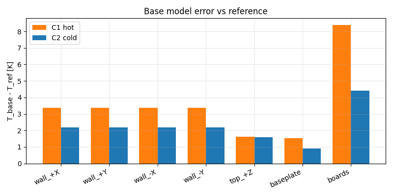
Base model: simulate and compare with the reference

Reusing the same model, we switch the parameters to the perturbed base values (c₀ = 0.5 · x_R), solve both load cases again, and plot the node error against the reference.

# Set the parameters to the BASE values and propagate to the network.
for name, value in zip(PARAM_NAMES, BASE):
    model.parameters.set_parameter(name, float(value))
tmm.formulas.apply_formulas()

# Resolve both load cases at BASE.
T_base_C1 = solve_case(CASES["C1"])
T_base_C2 = solve_case(CASES["C2"])

err_base_C1 = T_base_C1 - T_ref_C1
err_base_C2 = T_base_C2 - T_ref_C2

# --- Plot the node error vs reference ---
fig, ax = plt.subplots(figsize=(8, 4))
ax.bar(xpos - width / 2, err_base_C1, width, label="C1 hot", color="tab:orange")
ax.bar(xpos + width / 2, err_base_C2, width, label="C2 cold", color="tab:blue")
ax.axhline(0, color="k", lw=0.5)
ax.set_xticks(xpos)
ax.set_xticklabels(NODE_LABELS, rotation=25, ha="right")
ax.set_ylabel("T_base - T_ref [K]")
ax.set_title("Base model error vs reference")
ax.legend()
ax.grid(True, alpha=0.3)

plt.tight_layout()
plt.show()

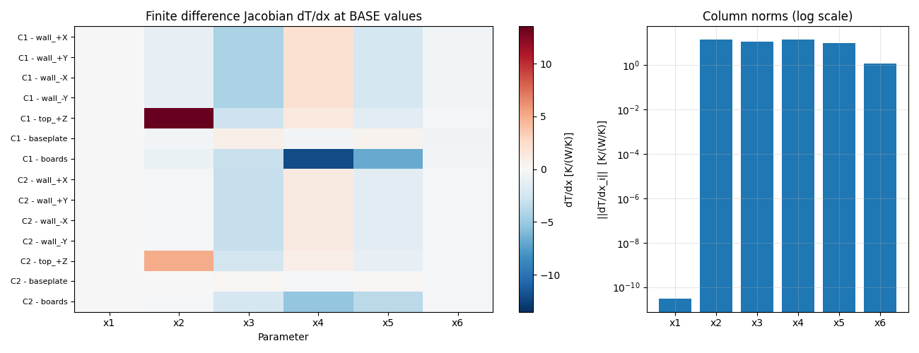
Steady-state sensitivities and the observability problem

We build the Jacobian dT/dx at the base values by forward finite differences against the SSLU solver: for each parameter x_i, perturb it by a small step h_i, resolve both load cases, and divide the temperature changes by h_i. The resulting matrix has 14 rows (7 nodes × 2 load cases) and 6 columns (one per parameter).

The heatmap and the column norms below show that the column of ``x1`` is essentially zero: the sidewall-sidewall couplings k12, k13, k34 produce no temperature change because load symmetry makes T1 = T2 = T3 = T4 and no heat flows through them. This is the observability problem discussed in the paper — and the reason the correlation in the next cell uses only Np = 5 free parameters (x2..x6).

# Compute the forward FD Jacobian at the BASE values for ALL 6 parameters,
# just for visualization (the actual correlation in the next cell uses Np=5).
def model_temperatures(x_full):
    for name, value in zip(PARAM_NAMES, x_full):
        model.parameters.set_parameter(name, float(value))
    tmm.formulas.apply_formulas()
    return np.concatenate([solve_case(CASES["C1"]), solve_case(CASES["C2"])])


FD_RELATIVE_STEP = 1e-2  # 1% forward step

T_at_base = model_temperatures(BASE)
J_full = np.zeros((T_at_base.size, BASE.size))
for i in range(BASE.size):
    h = FD_RELATIVE_STEP * max(abs(BASE[i]), 1.0)
    xp = BASE.copy()
    xp[i] = BASE[i] + h
    J_full[:, i] = (model_temperatures(xp) - T_at_base) / h

# Column norms (L2) make the observability problem visible in one number.
col_norms = np.linalg.norm(J_full, axis=0)

# --- Plot: heatmap of J and bar chart of column norms ---
fig, (ax1, ax2) = plt.subplots(1, 2, figsize=(13, 5), gridspec_kw={"width_ratios": [2, 1]})

vmax = np.max(np.abs(J_full))
row_labels = [f"C1 - {lbl}" for lbl in NODE_LABELS] + [f"C2 - {lbl}" for lbl in NODE_LABELS]
im = ax1.imshow(J_full, aspect="auto", cmap="RdBu_r", vmin=-vmax, vmax=vmax)
ax1.set_xticks(range(len(LABELS)))
ax1.set_xticklabels(LABELS)
ax1.set_yticks(range(len(row_labels)))
ax1.set_yticklabels(row_labels, fontsize=8)
ax1.set_xlabel("Parameter")
ax1.set_title("Finite difference Jacobian dT/dx at BASE values")
plt.colorbar(im, ax=ax1, label="dT/dx [K/(W/K)]")

ax2.bar(range(len(LABELS)), col_norms)
ax2.set_yscale("log")
ax2.set_xticks(range(len(LABELS)))
ax2.set_xticklabels(LABELS)
ax2.set_ylabel("||dT/dx_i||  [K/(W/K)]")
ax2.set_title("Column norms (log scale)")
ax2.grid(True, alpha=0.3, which="both")

plt.tight_layout()
plt.show()

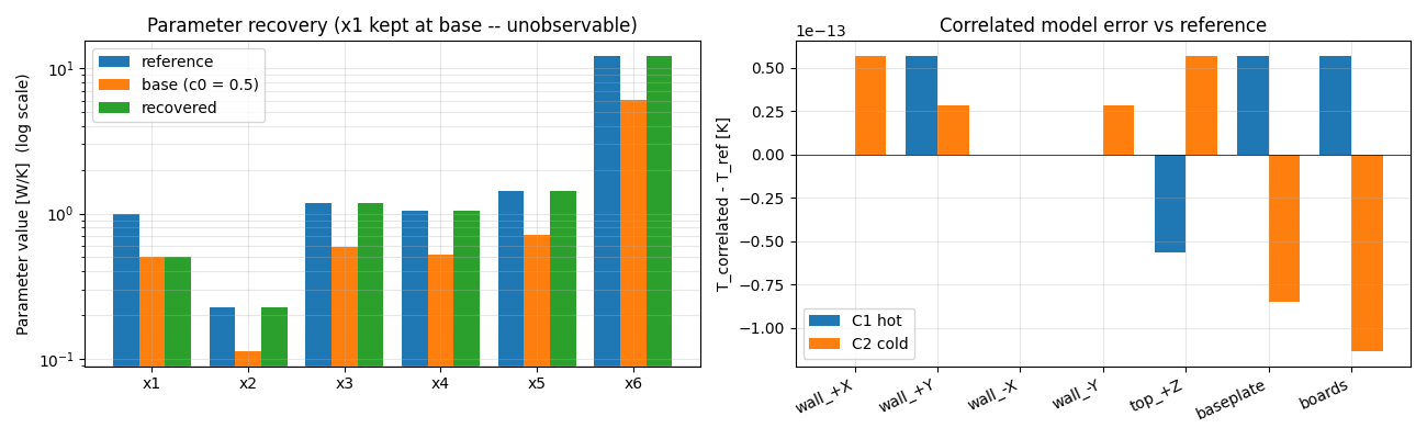
Correlation: recover the reference parameters

We define the residual vector (concatenated T_model − T_ref over the 7 diffusive nodes and the 2 load cases — 14 entries) and a forward FD Jacobian against the SSLU solver, and pass them to scipy.optimize.least_squares (trust-region reflective with non-negative bounds). Only x2..x6 are correlated; x1 is kept at its base value because it is unobservable from the temperature data.

Starting from c₀ = 0.5, the optimizer recovers the reference values. The node temperature error drops from a few K to numerical noise.

# Indices of the parameters that are actually correlated (drop x1 -- see above).
FREE_IDX = [1, 2, 3, 4, 5]
FREE_NAMES = [PARAM_NAMES[i] for i in FREE_IDX]
FREE_LABELS = [LABELS[i] for i in FREE_IDX]
FREE_REFERENCE = REFERENCE[FREE_IDX]
FREE_BASE = BASE[FREE_IDX]

T_REF_STACK = np.concatenate([T_ref_C1, T_ref_C2])


# Residual: concatenated (model - reference) over both cases, with only
# x2..x6 driven by the optimizer (x1 stays at its current value).
def residuals(x_free):
    for name, value in zip(FREE_NAMES, x_free):
        model.parameters.set_parameter(name, float(value))
    tmm.formulas.apply_formulas()
    return np.concatenate([solve_case(CASES["C1"]), solve_case(CASES["C2"])]) - T_REF_STACK


# Forward FD Jacobian over the 5 free parameters.
def jacobian(x_free):
    r0 = residuals(x_free)
    J = np.zeros((r0.size, x_free.size))
    for i in range(x_free.size):
        h = FD_RELATIVE_STEP * max(abs(x_free[i]), 1.0)
        xp = x_free.copy()
        xp[i] = x_free[i] + h
        J[:, i] = (residuals(xp) - r0) / h
    # Restore the model state to x_free for subsequent residual calls.
    for name, value in zip(FREE_NAMES, x_free):
        model.parameters.set_parameter(name, float(value))
    tmm.formulas.apply_formulas()
    return J


# Run the non-linear least-squares correlation (Np = 5).
result = least_squares(
    residuals,
    FREE_BASE.copy(),
    jac=jacobian,
    method="trf",
    bounds=(0.0, np.inf),
    xtol=1e-12,
    ftol=1e-12,
    gtol=1e-12,
)
recovered = result.x

# Evaluate the correlated model at the recovered parameters.
for name, value in zip(FREE_NAMES, recovered):
    model.parameters.set_parameter(name, float(value))
tmm.formulas.apply_formulas()
T_corr_C1 = solve_case(CASES["C1"])
T_corr_C2 = solve_case(CASES["C2"])
err_corr_C1 = T_corr_C1 - T_ref_C1
err_corr_C2 = T_corr_C2 - T_ref_C2

# --- Plot: parameter recovery (left), node temperature error (right) ---
fig, (ax1, ax2) = plt.subplots(1, 2, figsize=(13, 4))

# x1 keeps its BASE value (unobservable); the other five are recovered.
recovered_full = np.array([BASE[0]] + list(recovered))
pos = np.arange(len(LABELS))
w = 0.27
ax1.bar(pos - w, REFERENCE, w, label="reference")
ax1.bar(pos, BASE, w, label="base (c0 = 0.5)")
ax1.bar(pos + w, recovered_full, w, label="recovered")
ax1.set_yscale("log")
ax1.set_xticks(pos)
ax1.set_xticklabels(LABELS)
ax1.set_ylabel("Parameter value [W/K]  (log scale)")
ax1.set_title("Parameter recovery (x1 kept at base -- unobservable)")
ax1.legend()
ax1.grid(True, alpha=0.3, which="both")

ax2.bar(xpos - width / 2, err_corr_C1, width, label="C1 hot")
ax2.bar(xpos + width / 2, err_corr_C2, width, label="C2 cold")
ax2.axhline(0, color="k", lw=0.5)
ax2.set_xticks(xpos)
ax2.set_xticklabels(NODE_LABELS, rotation=25, ha="right")
ax2.set_ylabel("T_correlated - T_ref [K]")
ax2.set_title("Correlated model error vs reference")
ax2.legend()
ax2.grid(True, alpha=0.3)

plt.tight_layout()
plt.show()